Linear probing is a simple way to deal with collisions in a hash table. A collision happens when two items should go in the same spot. Imagine a parking lot where each car has a specific spot. If a car finds its spot taken, it moves down the line to find the next open one. That’s linear probing!
Let’s say we have 5 parking spots for cars numbered 1 to 5. Car 3 arrives and parks in spot 3. Then car 8 arrives. Spot 8 is outside our lot, so we loop back and start from spot 1, finding spot 3 taken. We check spot 4, and it’s open, so car 8 parks there. This way, all cars find a spot using linear probing.
Important Point on Linear Probing
- The simplest approach to resolve a collision is linear probing. In this technique, if a value is already stored at a location generated by h(k), it means collision occurred then we do a sequential search to find the empty location.
- Here the idea is to place a value in the next available position. Because in this approach searches are performed sequentially so it’s known as linear probing.
- Here array or hash table is considered circular because when the last slot reached an empty location not found then the search proceeds to the first location of the array.
Clustering is a major drawback of linear probing.
How Linear Probing Works?
Below is a hash function that calculates the next location. If the location is empty then store value otherwise find the next location.
Following hash function is used to resolve the collision in:
h(k, i) = [h(k) + i] mod m
Where
m = size of the hash table,
h(k) = (k mod m),
i = the probe number that varies from 0 to m–1.
Therefore, for a given key k, the first location is generated by [h(k) + 0] mod m, the first time i=0.
If the location is free, the value is stored at this location. If value successfully stores then probe count is 1 means location is founded on the first go.
If location is not free then second probe generates the address of the location given by [h(k) + 1]mod m.
Similarly, if the generated location is occupied, then subsequent probes generate the address as [h(k) + 2]mod m, [h(k) + 3]mod m, [h(k) + 4]mod m, [h(k) + 5]mod m, and so on, until a free location is found.
Probes is a count to find the free location for each value to store in the hash table.
Linear Probing Example
Insert the following sequence of keys in the hash table
{9, 7, 11, 13, 12, 8}
Use linear probing technique for collision resolution
h(k, i) = [h(k) + i] mod m
h(k) = 2k + 5
m=10
Solution:
Step 01:
First Draw an empty hash table of Size 10.
The possible range of hash values will be [0, 9].

Step 02:
Insert the given keys one by one in the hash table.
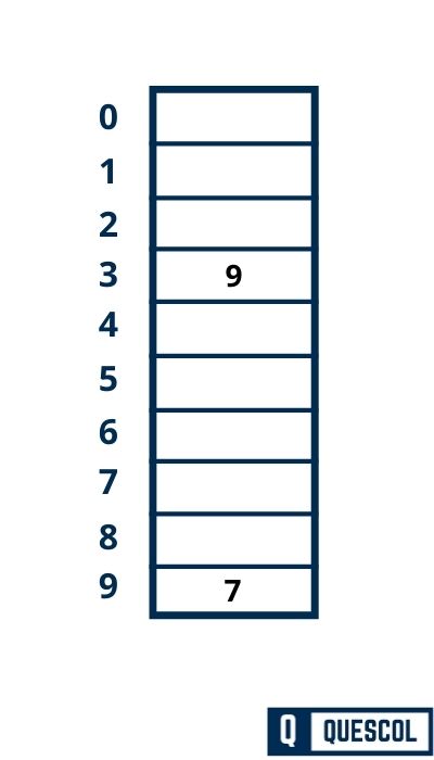
First Key to be inserted in the hash table = 9.
h(k) = 2k + 5
h(9) = 2*9 + 5 = 23
h(k, i) = [h(k) + i] mod m
h(9, 0) = [23 + 0] mod 10 = 3
So, key 9 will be inserted at index 3 of the hash table

Step 03:
Next Key to be inserted in the hash table = 7.
h(k) = 2k + 5
h(7) = 2*7 + 5 = 19
h(k, i) = [h(k) + i] mod m
h(7, 0) = [19 + 0] mod 10 = 9
So, key 7 will be inserted at index 9 of the hash table
Step 04:
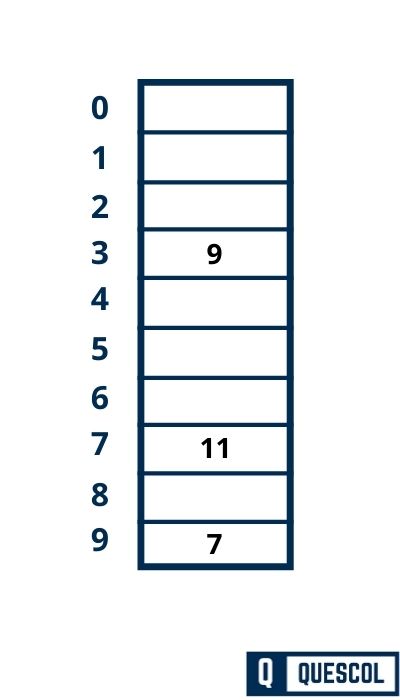
Next Key to be inserted in the hash table = 11.
h(k) = 2k + 5
h(11) = 2*11 + 5 = 27
h(k, i) = [h(k) + i] mod m
h(11, 0) = [27 + 0] mod 10 = 7
So, key 11 will be inserted at index 7 of the hash table
Step 05:
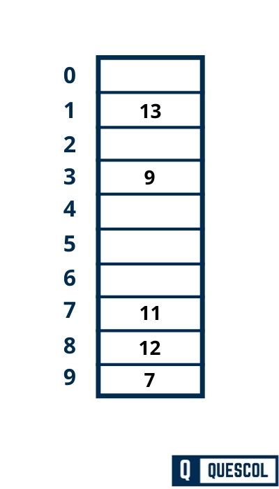
Next Key to be inserted in the hash table = 13.
h(k) = 2k + 5
h(13) = 2*13 + 5 = 31
h(k, i) = [h(k) + i] mod m
h(13, 0) = [31 + 0] mod 10 = 1
So, key 13 will be inserted at index 1 of the hash table

Step 06:
Next key to be inserted in the hash table = 12.
h(k) = 2k + 5
h(12) = 2*12 + 5 = 27
h(k, i) = [h(k) + i] mod m
h(12, 0) = [27 + 0] mod 10 = 7
Here Collision has occurred because index 7 is already filled.
Now we will increase i by 1.
h(12, 1) = [27 + 1] mod 10 = 8
So, key 12 will be inserted at index 8 of the hash table.
Step 07:
Next key to be inserted in the hash table = 8.
h(k) = 2k + 5
h(8) = 2*8 + 5 = 21
h(k, i) = [h(k) + i] mod m
h(8, 0) = [21 + 0] mod 10 = 1
Here Collision has occurred because index 1 is already filled.
Now we will increase i by 1 now i become 1.
h(k) = 2k + 5
h(8) = 2*8 + 5 = 21
h(k, i) = [h(k) + i] mod m
h(8, 0) = [21 + 1] mod 10 = 2
index 2 is vacant so 8 will be inserted at index 2.
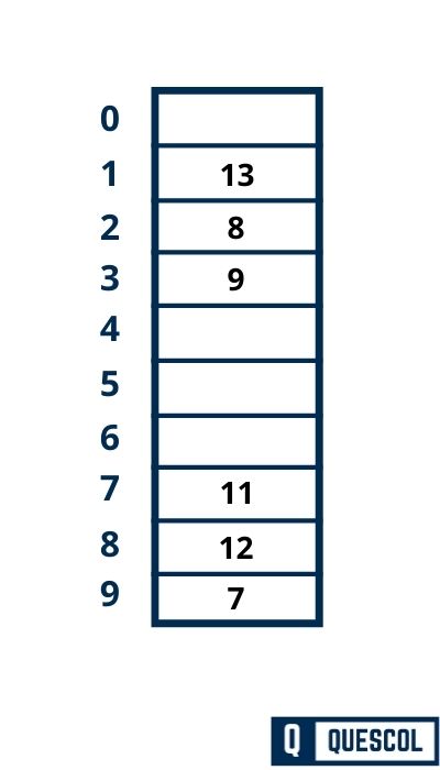
This is how the linear probing collision resolution technique works.
Challenges and Solutions in Linear Probing
- Clustering: One issue with linear probing is clustering, where a bunch of occupied spots clump together, slowing down the insertion and search processes. To minimize clustering, the table should have enough empty spots and use a good hash function that spreads items evenly.
- Infinite Loops: If the table gets full, linear probing could get stuck in an infinite loop. Ensuring the table never gets completely full or implementing a resizing mechanism can prevent this.
Real-world Example of Linear Probing
Imagine a classroom with lockers numbered 1 to 100, where students’ locker numbers are their birthdays modulo 100. If two students have the same birthday, the second student to arrive checks the next locker until finding an empty one.
For example, if two students have their birthday on January 1st (assuming it simplifies to locker number 1), and locker 1 is taken, the second student checks locker 2, 3, and so on, until they find an empty locker.
Efficiency and Use Cases of Linear Probing
Linear probing shines in situations where quick insertion and lookup times are critical, and the dataset does not frequently approach the hash table’s capacity. It’s used in various applications, from language interpreters and compilers to databases and caching systems.