The Floyd-Warshall algorithm is an algorithm that is used to find the shortest paths between all pairs of vertices in a weighted graph. This graph can be either directed or undirected. And the weights of the edges between two vertices can be positive, negative, or zero. However, the graph must not contain any negative weight cycles (cycles in the graph where the total weight is negative).
Floyd-Warshall algorithm basically follow the dynamic programming approach. It checks every possible path between the two vertices/nodes to calculate shortest distance between every pair of vertices/nodes.
Robert Floyd and Stephen Warshall created this algorithm. It’s very useful for things like GPS systems to find the best routes. It’s also used in computer networks to manage data flow. It helps to find the quickest way from one point to another.
Imagine you have a map of a few cities and the distances between them. This algorithm would look at all possible routes to find the shortest one between each pair of cities.
How Floyd Warshall Algorithm Work?
- Starting Off: We begin with a special table that shows how the points, or ‘vertices,’ ,’nodes’ in a graph are connected. If there is a direct path between two points, the table shows how long it is i.e. we put the value of the edge weight. If there isn’t a direct path, then we will put the really big number like infinite. And for the self vertices we put the 0.
- Making Updates: The algorithm checks every pair of points and tries to find if there’s a shorter path between them by going through another point. This process is repeated to make sure we find the shortest paths.
- Finishing Up: After checking all possible paths, the table will have the shortest distances between all the points.
Floyd Warshall Pseudocode
function FloydWarshall(graph):
    let dist be a |V| × |V| array of minimum distances initialized to Infinity
    for each vertex v
        dist[v][v] := 0
    for each edge (u,v)
        dist[u][v] := weight(u, v)
    for k from 1 to |V|
        for i from 1 to |V|
            for j from 1 to |V|
                if dist[i][k] + dist[k][j] < dist[i][j]
                    dist[i][j] := dist[i][k] + dist[k][j]
    return dist
Algorithm Steps
- Initialize: Start with the given matrix.
- Iterate for Each Vertex
k: For each pair of vertices(i, j), updatedist[i][j]tomin(dist[i][j], dist[i][k] + dist[k][j])
Example to understand Floyd Warshall Algorithm
Suppose we have a directed graph with four vertices (0, 1, 2, 3) and the following weighted edges:
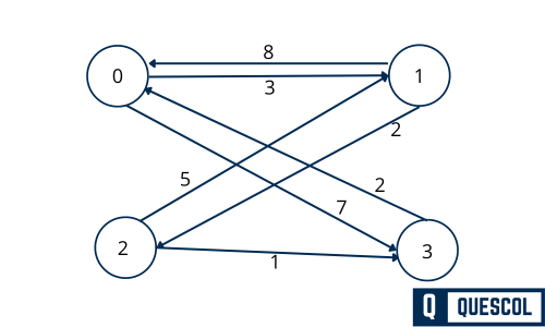
- Edge from 0 to 1 with weight 3
- Edge from 0 to 3 with weight 7
- Edge from 1 to 0 with weight 8
- Edge from 1 to 2 with weight 2
- Edge from 2 to 1 with weight 5
- Edge from 2 to 3 with weight 1
- Edge from 3 to 0 with weight 2
The graph’s adjacency matrix looks like this (using ∞ to represent no direct edge):
For Vertex 0
Using Vertex 0 as Intermediate:
- Evaluate paths through Vertex 0.
- Update
dist[i][j]tomin(dist[i][j], dist[i][0] + dist[0][j]). - For self node, value will be 0.
| 0 | 1 | 2 | 3 | |
|---|---|---|---|---|
| 0 | 0 | 3 | ∞ | 7 |
| 1 | 8 | 0 | ∞ | 15 |
| 2 | ∞ | 8 | 0 | 8 |
| 3 | 2 | 5 | ∞ | 0 |
For Vertex 1
In the above steps we have calculated the path from vertex 0. Now in this step we are checking if there is some shortest path if we consider vertex 1 as an intermediate vertex.
We’ll update each dist[i][j] to min(dist[i][j], dist[i][1] + dist[1][j]) for all pairs of vertices (i, j).
Given the current state of the matrix:
| 0 | 1 | 2 | 3 | |
|---|---|---|---|---|
| 0 | 0 | 3 | ∞ | 7 |
| 1 | 8 | 0 | ∞ | 15 |
| 2 | ∞ | 8 | 0 | 8 |
| 3 | 2 | 5 | ∞ | 0 |
Using Vertex 1 as Intermediate:
Each element of the matrix will be updated based on whether the path through Vertex 1 gives a shorter path between the pair of vertices:
- Update for
dist[0][2]:- Current value of
dist[0][2]is ∞. dist[0][1] + dist[1][2]is3 + 2 = 5.- Update
dist[0][2]tomin(∞, 5), which is5.
- Current value of
- Update for
dist[0][3]:- Current value of
dist[0][3]is7. dist[0][1] + dist[1][3]is3 + ∞ = ∞.- Update
dist[0][3]tomin(7, ∞), which is7.
- Current value of
- Update for
dist[2][0]:- Current value of
dist[2][0]is ∞. dist[2][1] + dist[1][0]is5 + 8 = 13.- Update
dist[2][0]tomin(∞, 13), which is13.
- Current value of
- Update for
dist[2][3]:- Current value of
dist[2][3]is1. dist[2][1] + dist[1][3]is5 + ∞ = ∞.- Update
dist[2][3]tomin(1, ∞), which is1.
- Current value of
- Update for
dist[3][0]:- Current value of
dist[3][0]is2. dist[3][1] + dist[1][0]is∞ + 8 = ∞.- Update
dist[3][0]tomin(2, ∞), which is2.
- Current value of
- Update for
dist[3][2]:- Current value of
dist[3][2]is ∞. dist[3][1] + dist[1][2]is∞ + 2 = ∞.- Update
dist[3][2]tomin(∞, ∞), which remains ∞.
- Current value of
Updated Matrix after applying above operation
After applying these updates using Vertex 1 as an intermediate vertex, the matrix becomes:
| 0 | 1 | 2 | 3 | |
|---|---|---|---|---|
| 0 | 0 | 3 | 5 | 7 |
| 1 | 8 | 0 | 2 | ∞ |
| 2 | 13 | 5 | 0 | 1 |
| 3 | 2 | ∞ | ∞ | 0 |
This matrix now contains updated shortest path distances between all pairs of vertices when considering vertex 1 as an intermediate step in the paths.
For Vertex 2
In the above steps we have calculated the path by consider vertex 1 as an intermediate vertex. Now in this step we are considering vertex 2 as intermediate and checking if there is possible shortest path.
We’ll calculate min(dist[i][j], dist[i][2] + dist[2][j]) for each pair of vertices (i, j).
Given the current state of the matrix:
| 0 | 1 | 2 | 3 | |
|---|---|---|---|---|
| 0 | 0 | 3 | 5 | 7 |
| 1 | 8 | 0 | 2 | ∞ |
| 2 | 13 | 5 | 0 | 1 |
| 3 | 2 | ∞ | ∞ | 0 |
Using Vertex 2 as Intermediate
- Update for
dist[0][3]:- Current value:
dist[0][3] = 7. - New possible value:
dist[0][2] + dist[2][3] = 5 + 1 = 6. - Update:
dist[0][3] = min(7, 6) = 6.
- Current value:
- Update for
dist[1][0]:- Current value:
dist[1][0] = 8. - New possible value:
dist[1][2] + dist[2][0] = 2 + 13 = 15. - No update needed since 8 < 15.
- Current value:
- Update for
dist[1][3]:- Current value:
dist[1][3] = ∞. - New possible value:
dist[1][2] + dist[2][3] = 2 + 1 = 3. - Update:
dist[1][3] = min(∞, 3) = 3.
- Current value:
- Update for
dist[3][0]:- Current value:
dist[3][0] = 2. - New possible value:
dist[3][2] + dist[2][0] = 7 + 13 = 20. - No update needed since 2 < 20.
- Current value:
- Update for
dist[3][1]:- Current value:
dist[3][1] = ∞. - New possible value:
dist[3][2] + dist[2][1] = 7 + 5 = 12. - Update:
dist[3][1] = min(∞, 12) = 12.
- Current value:
Updated Matrix after applying above operation
After applying these updates using Vertex 2 as an intermediate vertex, the matrix becomes:
| 0 | 1 | 2 | 3 | |
|---|---|---|---|---|
| 0 | 0 | 3 | 5 | 6 |
| 1 | 8 | 0 | 2 | 3 |
| 2 | 13 | 5 | 0 | 1 |
| 3 | 2 | 12 | 7 | 0 |
This matrix now reflects the shortest path distances between all pairs of vertices when considering vertex 2 as an intermediate step in the paths. The value of dist[i][j] represents the shortest distance from vertex i to vertex j after incorporating paths that pass through vertex 2.
For Vertex 3
In the above steps we have calculated the path by consider vertex 2 as an intermediate vertex. Now in this step we are considering vertex 3 as intermediate and checking if there is possible shortest path.
We’ll calculate min(dist[i][j], dist[i][3] + dist[3][j]) for each pair of vertices (i, j).
Given the current state of the matrix:
| 0 | 1 | 2 | 3 | |
|---|---|---|---|---|
| 0 | 0 | 3 | 5 | 6 |
| 1 | 5 | 0 | 2 | 3 |
| 2 | 4 | 5 | 0 | 1 |
| 3 | 2 | 5 | 6 | 0 |
Using Vertex 3 as Intermediate
- Update for
dist[0][1]:- Current value:
dist[0][1] = 3. - New possible value:
dist[0][3] + dist[3][1] = 6 + 5 = 11. - No update needed since 3 < 11.
- Current value:
- Update for
dist[0][2]:- Current value:
dist[0][2] = 5. - New possible value:
dist[0][3] + dist[3][2] = 6 + 6 = 12. - No update needed since 5 < 12.
- Current value:
- Update for
dist[1][0]:- Current value:
dist[1][0] = 5. - New possible value:
dist[1][3] + dist[3][0] = 3 + 2 = 5. - No update needed since they are equal.
- Current value:
- Update for
dist[1][2]:- Current value:
dist[1][2] = 2. - New possible value:
dist[1][3] + dist[3][2] = 3 + 6 = 9. - No update needed since 2 < 9.
- Current value:
- Update for
dist[2][0]:- Current value:
dist[2][0] = 4. - New possible value:
dist[2][3] + dist[3][0] = 1 + 2 = 3. - Update:
dist[2][0] = min(4, 3) = 3.
- Current value:
- Update for
dist[2][1]:- Current value:
dist[2][1] = 5. - New possible value:
dist[2][3] + dist[3][1] = 1 + 5 = 6. - No update needed since 5 < 6.
- Current value:
Updated Matrix after applying above operation
After applying these updates using Vertex 3 as an intermediate vertex, the matrix becomes:
| 0 | 1 | 2 | 3 | |
|---|---|---|---|---|
| 0 | 0 | 3 | 5 | 6 |
| 1 | 5 | 0 | 2 | 3 |
| 2 | 3 | 5 | 0 | 1 |
| 3 | 2 | 5 | 6 | 0 |
This matrix now represents the shortest path distances between all pairs of vertices when considering vertex 3 as an intermediate step in the paths. The value of dist[i][j] represents the shortest distance from vertex i to vertex j after incorporating paths that pass through vertex 3.